Bayes' rule

For the use of Bayes factor in model selection see Bayesian model selection

Bayesian statistics
Theory
Bayesian probability Probability interpretations Bayes' theorem Bayes' rule · Bayes factor Bayesian inference Bayesian network Prior · Posterior · Likelihood Conjugate prior Hyperparameter · Hyperprior Principle of indifference Principle of maximum entropy Empirical Bayes method Cromwell's rule Bernstein–von Mises theorem Bayesian information criterion Credible interval Maximum a posteriori estimation
Techniques
Bayesian linear regression Bayesian estimator Approximate Bayesian computation

In probability theory and applications, Bayes' rule relates the odds of event $A_1$ to event $A_2$ , before and after conditioning on event $B$ . The relationship is expressed in terms of the Bayes factor, $\Lambda$ . Bayes' rule is derived from and closely related to Bayes' theorem. Bayes' rule may be preferred over Bayes' theorem when the relative probability (that is, the odds) of two events matters, but the individual probabilities do not. This is because in Bayes' rule, $P(B)$ is eliminated and need not be calculated (see Derivation). It is commonly used in science and engineering, notably for model selection.

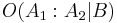Under the frequentist interpretation of probability, Bayes' rule is a general relationship between $O(A_1:A_2)$ and $O(A_1:A_2|B)$ , for any events $A_1$ , $A_2$ and $B$ in the same event space. In this case, $\Lambda$ represents the impact of the conditioning on the odds.

Under the Bayesian interpretation of probability, Bayes' rule relates the odds on probability models $A_1$ and $A_2$ before and after evidence $B$ is observed. In this case, $\Lambda$ represents the impact of the evidence on the odds. This is a form of Bayesian inference - the quantity $O(A_1:A_2)$ is called the prior odds, and $O(A_1:A_2|B)$ the posterior odds. By analogy to the prior and posterior probability terms in Bayes' theorem, Bayes' rule can be seen as Bayes' theorem in odds form. For more detail on the application of Bayes' rule under the Bayesian interpretation of probability, see Bayesian model selection.

1 The rule
- 1.1 Single event
- 1.2 Multiple events
2 Derivation
3 Examples
- 3.1 Frequentist example
- 3.2 Model selection
4 External links

The rule

Single event

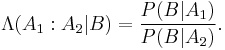
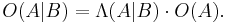
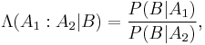
Given events $A_1$ , $A_2$ and $B$ , Bayes' rule states that the conditional odds of $A_1:A_2$ given $B$ are equal to the marginal odds of $A_1:A_2$ multiplied by the Bayes factor $\Lambda$ :

$O(A_1:A_2|B) = \Lambda(A_1:A_2|B) \cdot O(A_1:A_2) ,$

where

$\Lambda(A_1:A_2|B) = \frac{P(B|A_1)}{P(B|A_2)}.$

In the special case that $A_1 = A$ and $A_2 = \neg A$ , this may be written as

$O(A|B) = \Lambda(A|B) \cdot O(A) .$

Multiple events

Bayes' rule may be conditioned on an arbitrary number of events. For two events $B$ and $C$ ,

$O(A_1:A_2|B \cap C) = \Lambda(A_1:A_2|B \cap C) \cdot \Lambda(A_1:A_2|B) \cdot O(A_1:A_2) ,$

where

$\Lambda(A_1:A_2|B) = \frac{P(B|A_1)}{P(B|A_2)} ,$

$\Lambda(A_1:A_2|B \cap C) = \frac{P(C|A_1 \cap B)}{P(C|A_2 \cap B)} .$

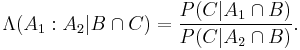
In this special case, the equivalent notation is

$O(A|B,C) = \Lambda(A|B \cap C) \cdot \Lambda(B|A) \cdot O(A).$

Derivation

Consider two instances of Bayes' theorem:

$P(A_1|B) = \frac{1}{P(B)} \cdot P(B|A_1) \cdot P(A_1),$

$P(A_2|B) = \frac{1}{P(B)} \cdot P(B|A_2) \cdot P(A_2).$

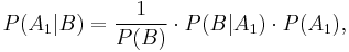
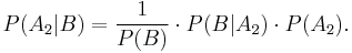
Combining these gives

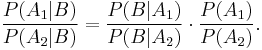
$\frac{P(A_1|B)}{P(A_2|B)} = \frac{P(B|A_1)}{P(B|A_2)} \cdot \frac{P(A_1)}{P(A_2)}.$

Now defining

$O(A_1:A_2|B) \triangleq \frac{P(A_1|B)}{P(A_2|B)}$

$O(A_1:A_2) \triangleq \frac{P(A_1)}{P(A_2)}$

$\Lambda(A_1:A_2|B) \triangleq \frac{P(B|A_1)}{P(B|A_2)},$

this implies

$O(A_1:A_2|B) = \Lambda(A_1:A_2|B) \cdot O(A_1:A_2).$

A similar derivation applies for conditioning on multiple events, using the appropriate extension of Bayes' theorem

Examples

Frequentist example

Consider the drug testing example in the article on Bayes' theorem.

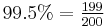The same results may be obtained using Bayes' rule. The prior odds on an individual being a drug-user are 199 to 1 against, as $\textstyle 0.5%=\frac{1}{200}$ and $\textstyle 99.5%=\frac{199}{200}$ . The Bayes factor when an individual tests positive is 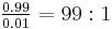$\textstyle \frac{0.99}{0.01} = 99:1$ in favour of being a drug-user: this is the ratio of the probability of a drug-user testing positive, to the probability of a non-drug user testing positive. The posterior odds on being a drug user are therefore $\textstyle 1 \times 99�: 199 \times 1 = 99:199$ , which is very close to 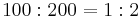$\textstyle 100:200 = 1:2$ . In round numbers, only one in three of those testing positive are actually drug-users.